Conditioning (probability)
Beliefs depend on the available information. This idea is formalized in probability theory by conditioning. Conditional probabilities, conditional expectations and conditional distributions are treated on three levels: discrete probabilities, probability density functions, and measure theory. Conditioning leads to a non-random result if the condition is completely specified; otherwise, if the condition is left random, the result of conditioning is also random.
This article concentrates on interrelations between various kinds of conditioning, shown mostly by examples. For systematic treatment (and corresponding literature) see more specialized articles mentioned below.
Contents |
Conditioning on the discrete level
Example. A fair coin is tossed 10 times; the random variable X is the number of heads in these 10 tosses, and Y — the number of heads in the first 3 tosses. In spite of the fact that Y emerges before X it may happen that someone knows X but not Y.
Conditional probability
Given that X = 1, the conditional probability of the event Y = 0 is P ( Y = 0 | X = 1 ) = P ( Y = 0, X = 1 ) / P ( X = 1 ) = 0.7. More generally,
for x = 0, 1, 2, 3, 4, 5, 6, 7; otherwise (for x = 8, 9, 10), P ( Y = 0 | X = x ) = 0. One may also treat the conditional probability as a random variable, — a function of the random variable X, namely,
The expectation of this random variable is equal to the (unconditional) probability,
namely,
which is an instance of the law of total probability E ( P ( A | X ) ) = P ( A ).
Thus, P ( Y = 0 | X = 1 ) may be treated as the value of the random variable P ( Y = 0 | X ) corresponding to X = 1. On the other hand, P ( Y = 0 | X = 1 ) is well-defined irrespective of other possible values of X.
Conditional expectation
Given that X = 1, the conditional expectation of the random variable Y is E ( Y | X = 1 ) = 0.3. More generally,
for x = 0, ..., 10. (In this example it appears to be a linear function, but in general it is nonlinear.) One may also treat the conditional expectation as a random variable, — a function of the random variable X, namely,
The expectation of this random variable is equal to the (unconditional) expectation of Y,
namely,
 or simply
which is an instance of the law of total expectation E ( E ( Y | X ) ) = E ( Y ).
The random variable E ( Y | X ) is the best predictor of Y given X. That is, it minimizes the mean square error E ( Y - f(X) )2 on the class of all random variables of the form f (X). This class of random variables remains intact if X is replaced, say, with 2X. Thus, E ( Y | 2X ) = E ( Y | X ). It does not mean that E ( Y | 2X ) = 0.3 × 2X; rather, E ( Y | 2X ) = 0.15 × 2X = 0.3 X. In particular, E ( Y | 2X=2 ) = 0.3. More generally, E ( Y | g(X) ) = E ( Y | X ) for every function g that is one-to-one on the set of all possible values of X. The values of X are irrelevant; what matters is the partition (denote it αX)
of the sample space Ω into disjoint sets  (Here
(Here  are all possible values of X.) Given an arbitrary partition α of Ω, one may define the random variable E ( Y | α ). Still, E ( E ( Y | α ) ) = E ( Y ).
Conditional probability may be treated as a special case of conditional expectation. Namely, P ( A | X ) = E ( Y | X ) if Y is the indicator of A. Therefore the conditional probability also depends on the partition αX generated by X rather than on X itself; P ( A | g(X) ) = P ( A | X ) = P ( A | α ), α = αX = αg(X).
On the other hand, conditioning on an event B is well-defined, provided that P ( B ) ≠ 0, irrespective of any partition that may contain B as one of several parts.
Conditional distribution
Given X = x, the conditional distribution of Y is
for 0 ≤ y ≤ min ( 3, x ). It is the hypergeometric distribution H ( x; 3, 7 ), or equivalently, H ( 3; x, 10-x ). The corresponding expectation 0.3 x, obtained from the general formula  for H ( n; R, W ), is nothing but the conditional expectation E ( Y | X = x ) = 0.3 x.
Treating H ( X; 3, 7 ) as a random distribution (a random vector in the four-dimensional space of all measures on {0,1,2,3}), one may take its expectation, getting the unconditional distribution of Y, — the binomial distribution Bin ( 3, 0.5 ). This fact amounts to the equality
for y = 0,1,2,3; just the law of total probability.
Conditioning on the level of densities
Example. A point of the sphere x2 + y2 + z2 = 1 is chosen at random according to the uniform distribution on the sphere [1] [2]. The random variables X, Y, Z are the coordinates of the random point. The joint density of X, Y, Z does not exist (since the sphere is of zero volume), but the joint density fX,Y of X, Y exists,
(The density is non-constant because of a non-constant angle between the sphere and the plane[3].) The density of X may be calculated by integration,
surprisingly, the result does not depend on x in (-1,1),
which means that X is distributed uniformly on (-1,1). The same holds for Y and Z (and in fact, for aX + bY + cZ whenever a2 + b2 + c2 = 1).
Conditional probability
Calculation
Given that X = 0.5, the conditional probability of the event Y ≤ 0.75 is the integral of the conditional density,
More generally,
for all x and y such that -1 < x < 1 (otherwise the denominator fX(x) vanishes) and  (otherwise the conditional probability degenerates to 0 or 1). One may also treat the conditional probability as a random variable, — a function of the random variable X, namely,
The expectation of this random variable is equal to the (unconditional) probability,
which is an instance of the law of total probability E ( P ( A | X ) ) = P ( A ).
Interpretation
The conditional probability P ( Y ≤ 0.75 | X = 0.5 ) cannot be interpreted as P ( Y ≤ 0.75, X = 0.5 ) / P ( X = 0.5 ), since the latter gives 0/0. Accordingly, P ( Y ≤ 0.75 | X = 0.5 ) cannot be interpreted via empirical frequencies, since the exact value X = 0.5 has no chance to appear at random, not even once during an infinite sequence of independent trials.
The conditional probability can be interpreted as a limit,
Conditional expectation
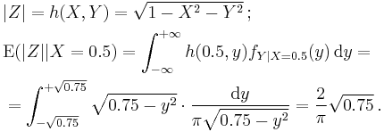
The conditional expectation E ( Y | X = 0.5 ) is of little interest; it vanishes just by symmetry. It is more interesting to calculate E ( |Z| | X = 0.5 ) treating |Z| as a function of X, Y:
More generally,
for -1 < x < 1. One may also treat the conditional expectation as a random variable, — a function of the random variable X, namely,
The expectation of this random variable is equal to the (unconditional) expectation of |Z|,
namely,
which is an instance of the law of total expectation E ( E ( Y | X ) ) = E ( Y ).
The random variable E ( |Z| | X ) is the best predictor of |Z| given X. That is, it minimizes the mean square error E ( |Z| - f(X) )2 on the class of all random variables of the form f (X). Similarly to the discrete case, E ( |Z| | g(X) ) = E ( |Z| | X ) for every measurable function g that is one-to-one on (-1,1).
Conditional distribution
Given X = x, the conditional distribution of Y, given by the density fY|X=x(y), is the (rescaled) arcsin distribution; its cumulative distribution function is
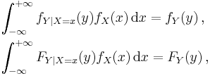
for all x and y such that x2 + y2 < 1.The corresponding expectation of h(x,Y) is nothing but the conditional expectation E ( h(X,Y) | X=x ). The mixture of these conditional distributions, taken for all x (according to the distribution of X) is the unconditional distribution of Y. This fact amounts to the equalities
the latter being the instance of the law of total probability mentioned above.
What conditioning is not
On the discrete level conditioning is possible only if the condition is of nonzero probability (one cannot divide by zero). On the level of densities, conditioning on X = x is possible even though P ( X = x ) = 0. This success may create the illusion that conditioning is always possible. Regretfully, it is not, for several reasons presented below.
Geometric intuition: caution
The result P ( Y ≤ 0.75 | X = 0.5 ) = 5/6, mentioned above, is geometrically evident in the following sense. The points (x,y,z) of the sphere x2 + y2 + z2 = 1, satisfying the condition x = 0.5, are a circle y2 + z2 = 0.75 of radius  on the plane x = 0.5. The inequality y ≤ 0.75 holds on an arc. The length of the arc is 5/6 of the length of the circle, which is why the conditional probability is equal to 5/6.
This successful geometric explanation may create the illusion that the following question is trivial.
- A point of a given sphere is chosen at random (uniformly). Given that the point lies on a given plane, what is its conditional distribution?
It may seem evident that the conditional distribution must be uniform on the given circle (the intersection of the given sphere and the given plane). Sometimes it really is, but in general it is not. Especially, Z is distributed uniformly on (-1,+1) and independent of the ratio Y/X, thus, P ( Z ≤ 0.5 | Y/X ) = 0.75. On the other hand, the inequality z ≤ 0.5 holds on an arc of the circle x2 + y2 + z2 = 1, y = cx (for any given c). The length of the arc is 2/3 of the length of the circle. However, the conditional probability is 3/4, not 2/3. This is a manifestation of the classical Borel paradox.[4][5]
Appeals to symmetry can be misleading if not formalized as invariance arguments.—Pollard[6]
Another example. A random rotation of the three-dimensional space is a rotation by a random angle around a random axis. Geometric intuition suggests that the angle is independent of the axis and distributed uniformly. However, the latter is wrong; small values of the angle are less probable.
The limiting procedure
Given an event B of zero probability, the formula  is useless, however, one can try
  for an appropriate sequence of events Bn of nonzero probability such that Bn ↓ B (that is,
  and
and  ). One example is given above. Two more examples are Brownian bridge and Brownian excursion.
In the latter two examples the law of total probability is irrelevant, since only a single event (the condition) is given. In contrast, in the example above the law of total probability applies, since the event X = 0.5 is included into a family of events X = x where x runs over (-1,1), and these events are a partition of the probability space.
In order to avoid paradoxes (such as the Borel's paradox), the following important distinction should be taken into account. If a given event is of nonzero probability then conditioning on it is well-defined (irrespective of any other events), as was noted above. In contrast, if the given event is of zero probability then conditioning on it is ill-defined unless some additional input is provided. Wrong choice of this additional input leads to wrong conditional probabilities (expectations, distributions). In this sense, "the concept of a conditional probability with regard to an isolated hypothesis whose probability equals 0 is inadmissible." (Kolmogorov; quoted in [6]).
The additional input may be (a) a symmetry (invariance group); (b) a sequence of events Bn such that Bn ↓ B, P ( Bn ) > 0; (c) a partition containing the given event. Measure-theoretic conditioning (below) investigates Case (c), discloses its relation to (b) in general and to (a) when applicable.
Some events of zero probability are beyond the reach of conditioning. An example: let Xn be independent random variables distributed uniformly on (0,1), and B the event "Xn → 0 as  "; what about P ( Xn < 0.5 | B ) ? Does it tend to 1, or not? Another example: let X be a random variable distributed uniformly on (0,1), and B the event "X is a rational number"; what about P ( X = 1/n | B ) ? The only answer is that, once again,
the concept of a conditional probability with regard to an isolated hypothesis whose probability equals 0 is inadmissible.—Kolmogorov, quoted in [6]
Conditioning on the level of measure theory
Example. Let Y be a random variable distributed uniformly on (0,1), and X = f(Y) where f is a given function. Two cases are treated below: f = f1 and f = f2, where f1 is the continuous piecewise-linear function
and f2 is the Weierstrass function.
Geometric intuition: caution
Given X = 0.75, two values of Y are possible, 0.25 and 0.5. It may seem evident that both values are of conditional probability 0.5 just because one point is congruent to another point. However, this is an illusion; see below.
Conditional probability
The conditional probability P ( Y ≤ 1/3 | X ) may be defined as the best predictor of the indicator
given X. That is, it minimizes the mean square error E ( I - g(X) )2 on the class of all random variables of the form g (X).
In the case f = f1 the corresponding function g = g1 may be calculated explicitly,[details 1]
Alternatively, the limiting procedure may be used,
giving the same result.
Thus, P ( Y ≤ 1/3 | X ) = g1 (X). The expectation of this random variable is equal to the (unconditional) probability, E ( P ( Y ≤ 1/3 | X ) ) = P ( Y ≤ 1/3 ), namely,
which is an instance of the law of total probability E ( P ( A | X ) ) = P ( A ).
In the case f = f2 the corresponding function g = g2 probably cannot be calculated explicitly. Nevertheless it exists, and can be computed numerically. Indeed, the space L2 (Ω) of all square integrable random variables is a Hilbert space; the indicator I is a vector of this space; and random variables of the form g (X) are a (closed, linear) subspace. The orthogonal projection of this vector to this subspace is well-defined. It can be computed numerically, using finite-dimensional approximations to the infinite-dimensional Hilbert space.
Once again, the expectation of the random variable P ( Y ≤ 1/3 | X ) = g2 (X) is equal to the (unconditional) probability, E ( P ( Y ≤ 1/3 | X ) ) = P ( Y ≤ 1/3 ), namely,
However, the Hilbert space approach treats g2 as an equivalence class of functions rather than an individual function. Measurability of g2 is ensured, but continuity (or even Riemann integrability) is not. The value g2 (0.5) is determined uniquely, since the point 0.5 is an atom of the distribution of X. Other values x are not atoms, thus, corresponding values g2 (x) are not determined uniquely. Once again, "the concept of a conditional probability with regard to an isolated hypothesis whose probability equals 0 is inadmissible." (Kolmogorov; quoted in [6]).
Alternatively, the same function g (be it g1 or g2) may be defined as the Radon–Nikodym derivative
where measures μ, ν are defined by
for all Borel sets  That is, μ is the (unconditional) distribution of X, while ν is one third of its conditional distribution,
Both approaches (via the Hilbert space, and via the Radon–Nikodym derivative) treat g as an equivalence class of functions; two functions g and g′ are treated as equivalent, if g (X) = g′ (X) almost surely. Accordingly, the conditional probability P ( Y ≤ 1/3 | X ) is treated as an equivalence class of random variables; as usual, two random variables are treated as equivalent if they are equal almost surely.
Conditional expectation
The conditional expectation E ( Y | X ) may be defined as the best predictor of Y given X. That is, it minimizes the mean square error E ( Y - h(X) )2 on the class of all random variables of the form h(X).
In the case f = f1 the corresponding function h = h1 may be calculated explicitly,[details 2]
Alternatively, the limiting procedure may be used,
giving the same result.
Thus, E ( Y | X ) = h1 (X). The expectation of this random variable is equal to the (unconditional) expectation, E ( E ( Y | X ) ) = E ( Y ), namely,
which is an instance of the law of total expectation E ( E ( Y | X ) ) = E ( Y ).
In the case f = f2 the corresponding function h = h2 probably cannot be calculated explicitly. Nevertheless it exists, and can be computed numerically in the same way as g2 above, — as the orthogonal projection in the Hilbert space. The law of total expectation holds, since the projection cannot change the scalar product by the constant 1 belonging to the subspace.
Alternatively, the same function h (be it h1 or h2) may be defined as the Radon–Nikodym derivative
where measures μ, ν are defined by
for all Borel sets  Here E ( Y; A ) is the restricted expectation, not to be confused with the conditional expectation E ( Y | A ) = E (Y; A ) / P ( A ).
Conditional distribution
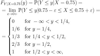
In the case f = f1 the conditional cumulative distribution function may be calculated explicitly, similarly to g1. The limiting procedure gives
which cannot be correct, since a cumulative distribution function must be right-continuous!
This paradoxical result is explained by measure theory as follows. For a given y the corresponding FY|X=x(y) = P ( Y ≤ y | X = x ) is well-defined (via the Hilbert space or the Radon–Nikodym derivative) as an equivalence class of functions (of x). Treated as a function of y for a given x it is ill-defined unless some additional input is provided. Namely, a function (of x) must be chosen within every (or at least almost every) equivalence class. Wrong choice leads to wrong conditional cumulative distribution functions.
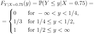
A right choice can be made as follows. First, FY|X=x(y) = P ( Y ≤ y | X = x ) is considered for rational numbers y only. (Any other dense countable set may be used equally well.) Thus, only a countable set of equivalence classes is used; all choices of functions within these classes are mutually equivalent, and the corresponding function of rational y is well-defined (for almost every x). Second, the function is extended from rational numbers to real numbers by right continuity.
In general the conditional distribution is defined for almost all x (according to the distribution of X), but sometimes the result is continuous in x, in which case individual values are acceptable. In the considered example this is the case; the correct result for x = 0.75,
shows that the conditional distribution of Y given X = 0.75 consists of two atoms, at 0.25 and 0.5, of probabilities 1/3 and 2/3 respectively.
Similarly, the conditional distribution may be calculated for all x in (0, 0.5) or (0.5, 1).
The value x = 0.5 is an atom of the distribution of X, thus, the corresponding conditional distribution is well-defined and may be calculated by elementary means (the denominator does not vanish); the conditional distribution of Y given X = 0.5 is uniform on (2/3, 1). Measure theory leads to the same result.
The mixture of all conditional distributions is the (unconditional) distribution of Y.
The conditional expectation E ( Y | X = x ) is nothing but the expectation with respect to the conditional distribution.
In the case f = f2 the corresponding FY|X=x(y) = P ( Y ≤ y | X = x ) probably cannot be calculated explicitly. For a given y it is well-defined (via the Hilbert space or the Radon–Nikodym derivative) as an equivalence class of functions (of x). The right choice of functions within these equivalence classes may be made as above; it leads to correct conditional cumulative distribution functions, thus, conditional distributions. In general, conditional distributions need not be atomic or absolutely continuous (nor mixtures of both types). Probably, in the considered example they are singular (like the Cantor distribution).
Once again, the mixture of all conditional distributions is the (unconditional) distribution, and the conditional expectation is the expectation with respect to the conditional distribution.
Technical details
- ^ Proof:
- ^ Proof:
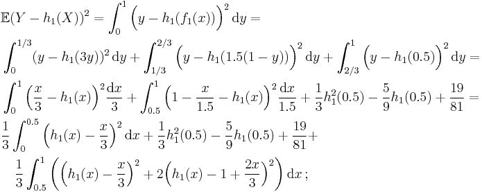 it remains to note that
  is minimal at
  and
and  is minimal at
See also
- Conditional probability
- Conditional expectation
- Conditional probability distribution
- Joint probability distribution
- Borel's paradox
- Regular conditional probability
- Disintegration theorem
- Law of total variance
- Law of total cumulance
Notes
- ^ n-sphere#Generating points on the surface of the n-ball
- ^ wikibooks: Uniform Spherical Distribution
- ^ Area#General formula
- ^ Pollard 2002, Sect. 5.5, Example 17 on page 122
- ^ Durrett 1996, Sect. 4.1(a), Example 1.6 on page 224
- ^ a b c d Pollard 2002, Sect. 5.5, page 122
References
- Durrett, Richard (1996), Probability: theory and examples (Second ed.)
- Pollard, David (2002), A user's guide to measure theoretic probability, Cambridge University Press


